欧博ABG官网-欧博官方网址-会员登入

TLDR

Step 1

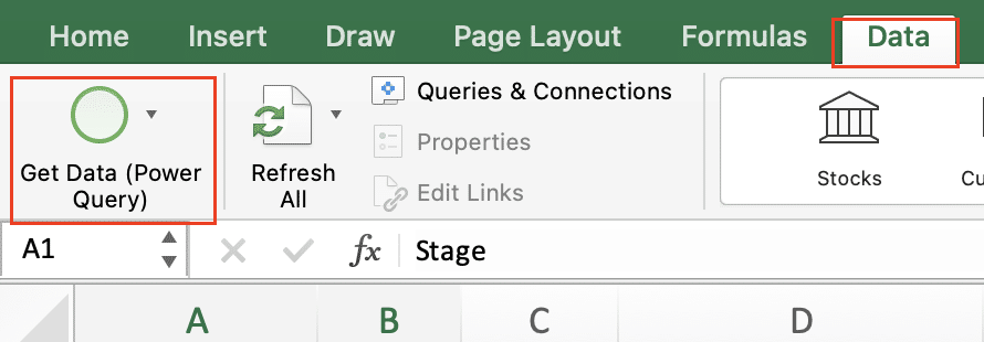
Open Excel and go to the Data tab. Look for the “Get Data” button in the ribbon.

Step 2

Click “Get Data” to see a dropdown menu of options. Choose your data source (e.g., Excel workbook, CSV file, database).

Step 3

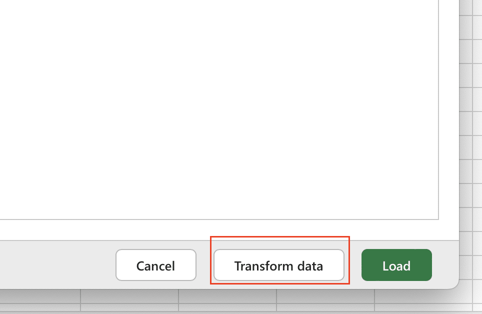
Browse to locate your file and select it. A preview window will appear. Review the data and click “Load” to import it directly, or “Transform Data” to open the Power Query Editor.

Step 4

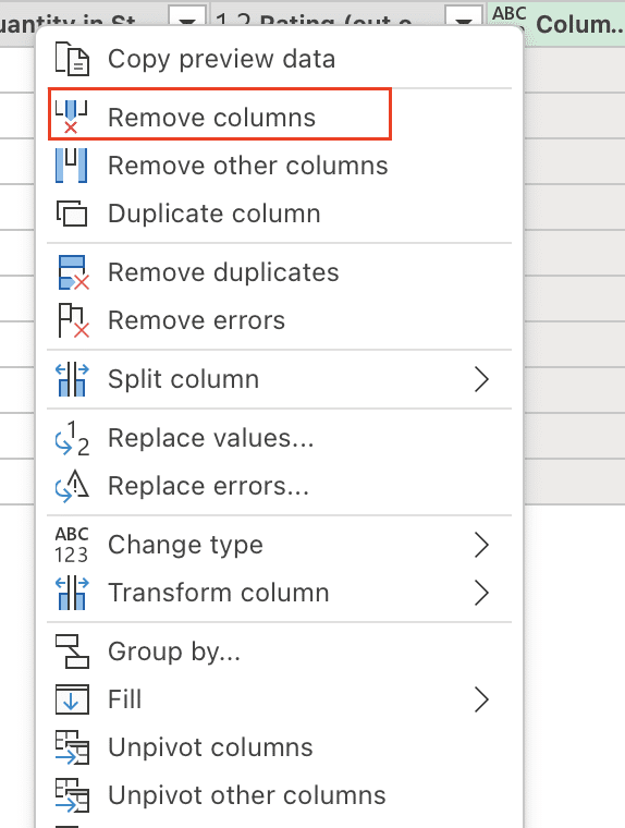
If you clicked “Transform Data,” the Power Query Editor will open automatically. In the Power Query Editor, you can now start cleaning your data. To remove a column, right-click on the column header and select “Remove.” To change a data type, click on the icon next to the column name and choose the appropriate type.

Step 5

Once you’re satisfied with your changes, click “Close & Load” in the Home tab. Your transformed data will now appear in a new sheet in your Excel workbook.

Want to transform and clean data in Excel quickly? Power Query is your answer. This guide walks you through using Power Query, from basic imports to advanced techniques.

Creating Your First Power Query in Excel

Power Query allows you to import, transform, and load data efficiently. Here’s how to get started:

Step 1: Access Power Query

Open Excel and go to the Data tab.

Look for the “Get Data” button in the ribbon.

Step 2: Select Your Data Source

Click “Get Data” to see a dropdown menu of options.

Choose your data source (e.g., Excel workbook, CSV file, database).

For this example, let’s use an Excel workbook.

Step 3: Import the Data

Browse to locate your file and select it.

A preview window will appear. Review the data and click “Load” to import it directly, or “Transform Data” to open the Power Query Editor.

Step 4: Open the Power Query Editor

If you clicked “Transform Data,” the Power Query Editor will open automatically.

This is where you’ll perform your data transformations.

Step 5: Apply Basic Transformations

In the Power Query Editor, you can now start cleaning your data.

To remove a column, right-click on the column header and select “Remove.”

To change a data type, click on the icon next to the column name and choose the appropriate type.

Step 6: Load Transformed Data

Once you’re satisfied with your changes, click “Close & Load” in the Home tab.

Your transformed data will now appear in a new sheet in your Excel workbook.

How to Transform Data Using Power Query

Power Query offers numerous ways to clean and reshape your data. Let’s explore some common transformations:

Removing Duplicate Rows

Duplicate data can skew your analysis. Here’s how to remove them:

Step 1: Select Columns

In the Power Query Editor, hold Ctrl and click on the column headers you want to check for duplicates.

Step 2: Remove Duplicates

Go to the Home tab in the Power Query Editor.

Click on “Remove Rows.”

From the dropdown, select “Remove Duplicates.”

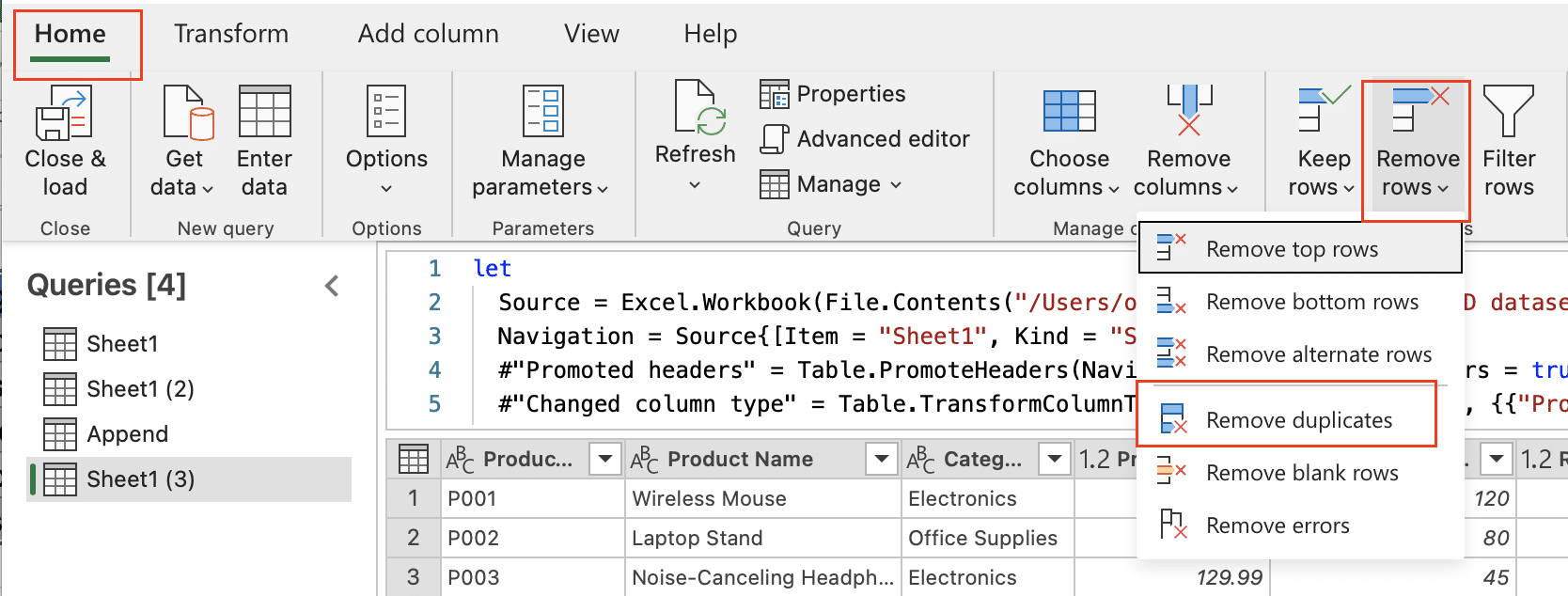
Power Query will then remove all but the first instance of any duplicate rows based on the columns you selected.

Merging Multiple Tables

Combining data from different sources is a powerful feature of Power Query:

Step 1: Import Tables

Import all relevant tables into Power Query as separate queries.

Step 2: Start the Merge Process

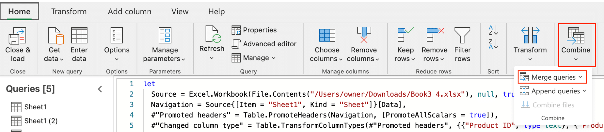
Select one of your queries in the Queries pane.

Click “Combine > Merge Queries” in the Home tab.

Step 3: Choose Tables and Join Columns

In the Merge window, select the second table you want to join.

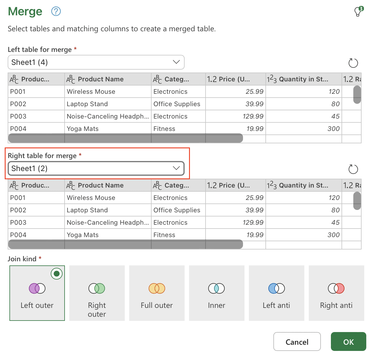
Choose the columns from each table that you want to use for the join.

These columns should contain the same type of data (e.g., customer IDs).

Step 4: Select Join Type

Choose the appropriate join type:

Left Outer: Keep all rows from the first table, matching rows from the second.

Inner: Keep only rows that exist in both tables.

Full Outer: Keep all rows from both tables.

Right Outer: Keep all rows from the second table, matching rows from the first.

Step 5: Finalize the Merge

Click OK to complete the merge.

The result will be a new column in your original query with data from the second table.

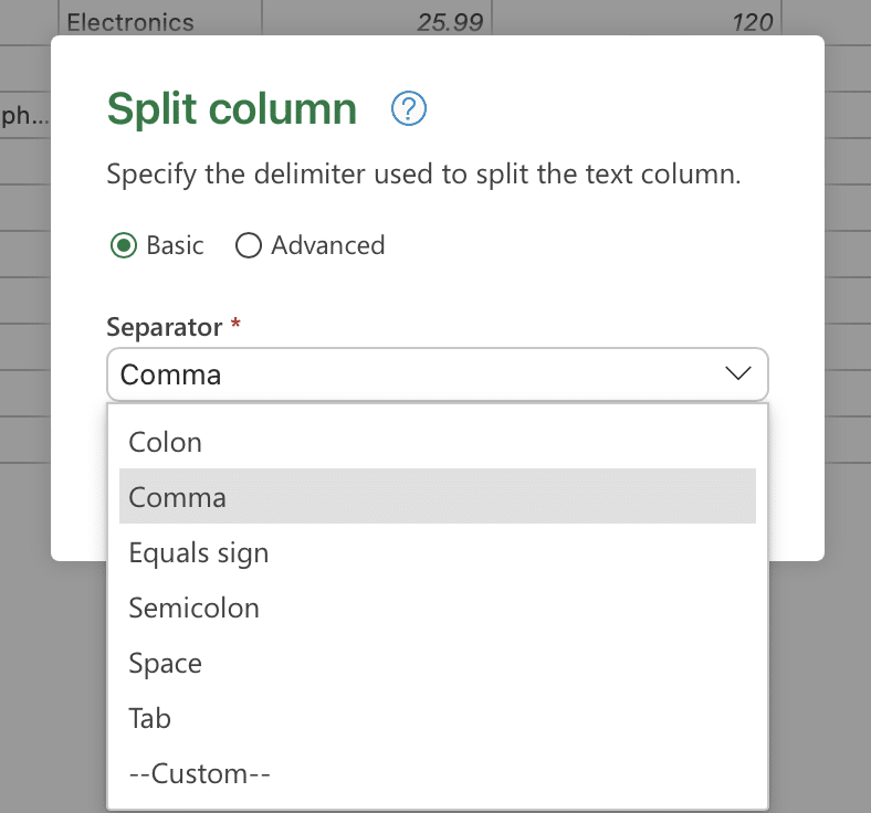
Splitting Columns

Sometimes you need to separate data within a single column:

Step 1: Select the Column

Click on the column header you want to split.

Step 2: Choose Split Method

Go to the Transform tab.

Click “Split Column.”

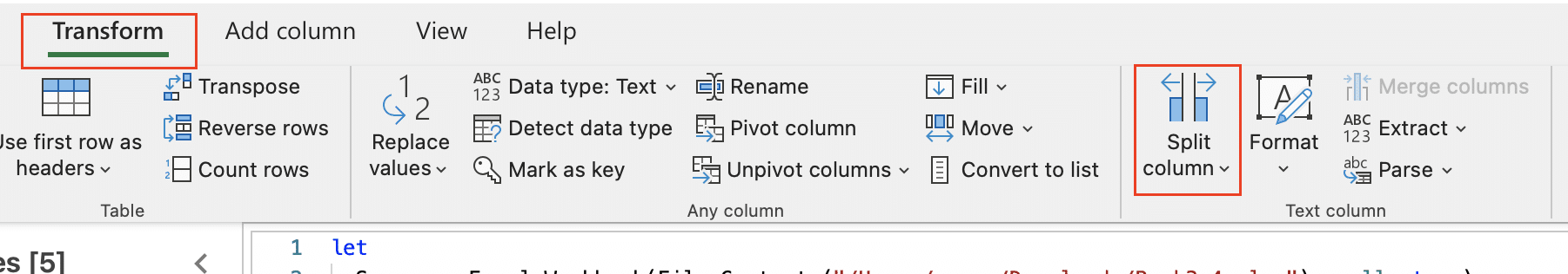
Choose “By Delimiter” if splitting based on a character, or “By Number of Characters” for fixed-width data.

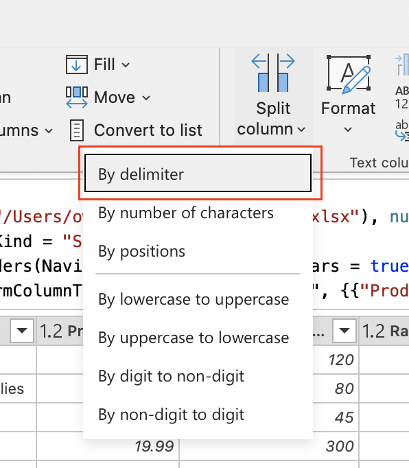
Step 3: Set Split Options

For delimiter splits, enter the character(s) used to separate the data.

For character number splits, specify how many characters should be in each new column.

Step 4: Apply the Split

Click OK to split the column.

Power Query will create new columns with the split data.

How Do You Enter a Power Query in Excel?

While the graphical interface is user-friendly, you can also write queries directly:

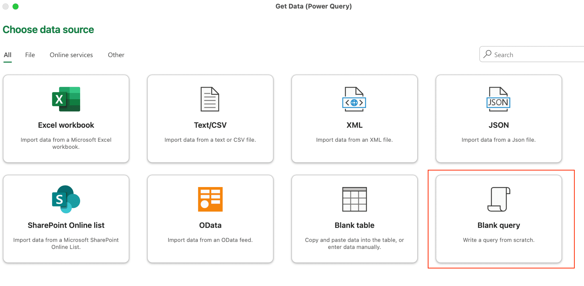
Step 1: Create a Blank Query

Go to Data > Get Data > From Other Sources > Blank Query.

Step 2: Open Advanced Editor

In the Power Query Editor, go to the Home tab.

Click on “Advanced Editor.”

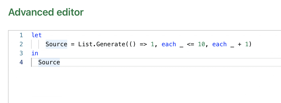
Step 3: Enter Your M Formula

In the Advanced Editor window, you can write your M language formula.

For example, to create a list of numbers from 1 to 10:
Copy
let

Try the Free Spreadsheet Extension Over 500,000 Pros Are Raving About

Stop exporting data manually. Sync data from your business systems into Google Sheets or Excel with Coefficient and set it on a refresh schedule.

Get Started

Source = List.Generate(() => 1, each _ <= 10, each _ + 1)

in

Source

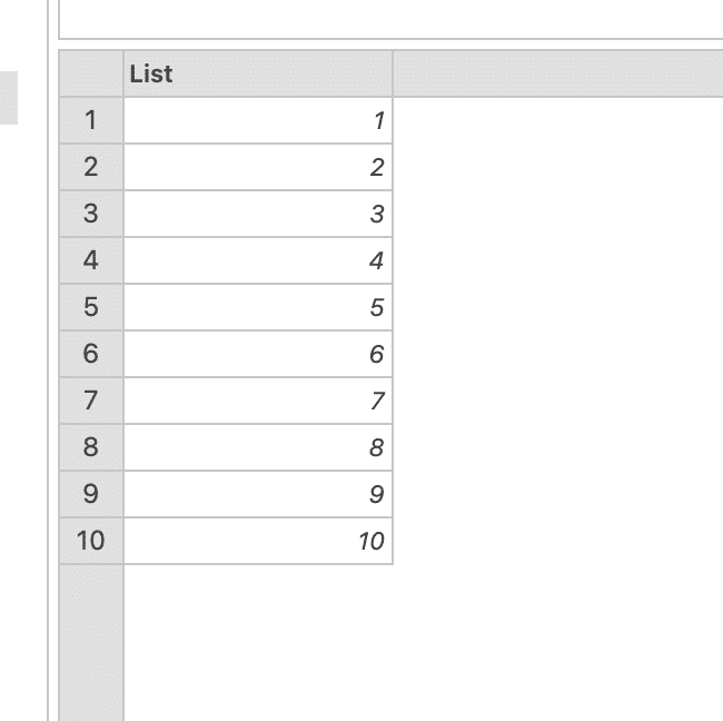
Step 4: Apply and Refine

Click “Done” to apply your formula.

Review the results and adjust your query as needed.

Advanced Power Query Techniques

Once you’re comfortable with the basics, try these advanced techniques:

Creating Custom Functions

Custom functions allow you to reuse complex transformations:

Step 1: Open a Blank Query

Go to Get Data > Blank Query.

Step 2: Write Your Function

Open the Advanced Editor.

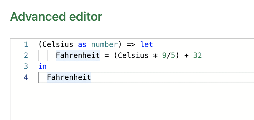
Write your function in M language. For example, a function to convert Celsius to Fahrenheit:
Copy
(Celsius as number) => let

Fahrenheit = (Celsius * 9/5) + 32

in

Fahrenheit

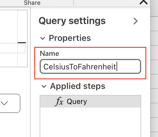
Step 3: Save the Function

Name your query (e.g., “CelsiusToFahrenheit”).

Right-click on the query and select “Create Function.”

Step 4: Use Your Function

In other queries, you can now call your function:
Copy
= CelsiusToFahrenheit([Temperature])

Using Parameters in Queries

Parameters make your queries more flexible:

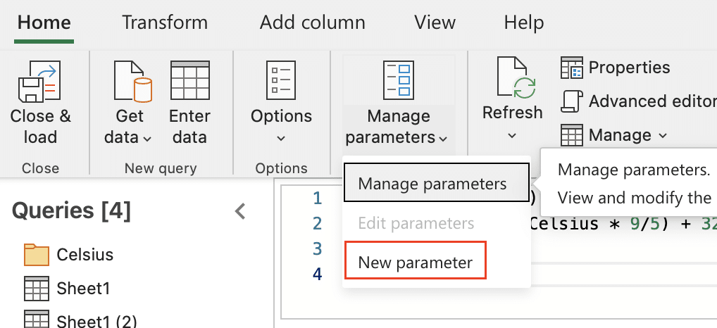
Step 1: Create a Parameter

Go to Manage Parameters > New Parameter.

Set a name, type, and current value for your parameter.

Step 2: Use the Parameter

In your queries, reference the parameter using @ParameterName.

For example, to filter data based on a date parameter:
Copy
= Table.SelectRows(YourTable, each [Date] > @StartDate)

Step 3: Update Parameters

Change parameter values to dynamically adjust your query results.

Handling Errors and Null Values

Robust queries need good error handling:

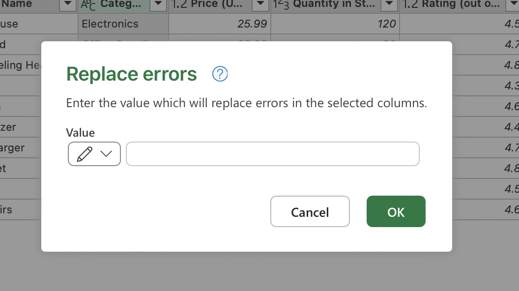
Step 1: Replace Errors

Select a column with errors.

Go to Transform > Replace Values > Replace Error.

Choose a replacement value (e.g., 0 or “Unknown”).

Step 2: Fill Null Values

For columns with null values, go to Transform > Fill.

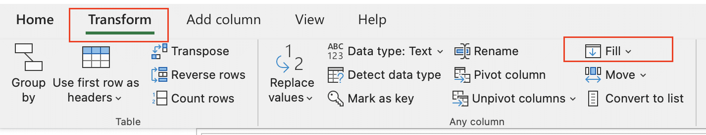
Choose to fill up, down, or with a specific value.

Step 3: Use Error Handling in Formulas

In custom formulas, use try/otherwise for error handling:
Copy
= try Number.FromText([Amount]) otherwise 0

Mastering Power Query for Efficient Data Management

By learning Power Query, you’ve gained a powerful tool for data transformation in Excel. Keep practicing these techniques to streamline your data workflows and enhance your analysis capabilities.

Ready to take your data management to the next level? Try Coefficient to seamlessly sync live data from various business systems into your spreadsheets. Get started with Coefficient today and experience effortless data integration.